S-Parameter Viewer User Guide

User Guide

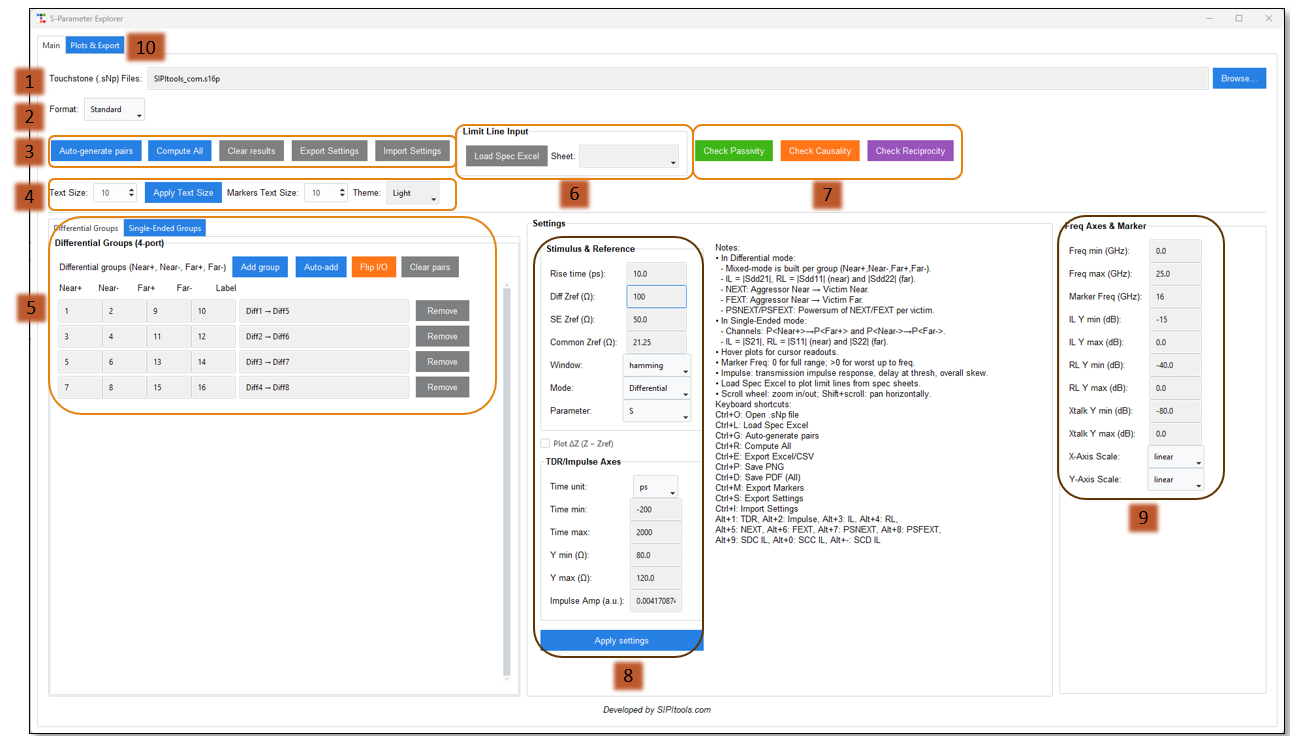
1.0 The prompt allows you to load multiple S-parameter files for analysis and plot them concurrently, facilitating direct comparison across datasets.

2.0 The Format section offers multiple options: Standard, OEM, and Auto modes.

2.1 Standard Format:
For an S4P file, the inputs are Port 1 and Port 2, and the outputs are Port 3 and Port 4.

2.2 OEM Format:
For an S4P file, the inputs are Port 1 and Port 3, and the outputs are Port 2 and Port 4.

2.3 Auto Mode:
Inputs and outputs are automatically determined.

3.0 These options allow you to auto-generate port mappings, compute results, and manage settings.

3.1 Auto-Generate Pairs:
Automatically assigns input and output ports and generates differential pairs based on the selected format.

3.2 Compute All:
Recomputes results after using Auto-Generate Pairs, switching to single-ended mode (default is differential), or making any configuration changes.

3.3 Clear Results:
Clears all currently displayed results.

3.4 Import/Export Settings:
Enables importing or exporting the current plotting configuration for reuse or sharing.

4.0 This window allows you to customize text sizes and themes.

4.1 Text Size:

Adjusts the overall text size throughout the tool, excluding marker and legend text.

4.2 Marker Text Size:

Controls the text size for markers and their associated legends.

4.3 Theme:

Allows you to switch between Light and Dark themes based on your preference.

5.0 The Single-Ended/Differential Group window allows you to add or delete groups and flip input/output port assignments.

5.1 Auto-Add:
Automatically assigns input and output ports and creates differential pairs based on the selected format.

5.2 Add Group:
Allows you to manually specify input and output ports for single-ended or differential signals.

5.3 Flip I/O:
Flips the assigned input and output ports. This is especially useful when plotting NEXT, PSNEXT, FEXT, and PSFEXT, allowing you to view crosstalk from both ends.

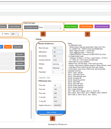
6.0 Limit Line Input

6.1 Load Spec Excel:
Allows you to load a specification defined in an Excel file. Typically, Column 1 contains frequency values, while Column 2 contains magnitude (or other relevant parameters).

6.2 Multiple Sheets Support:
An Excel file may contain multiple sheets, each representing different specifications such as IL, RL, or crosstalk. For example, Sheet 1 may include PCIe Gen5 specifications, while Sheet 2 may contain PCIe Gen6 specifications.

7.0 Passivity, Causality & Reciprocity Checks

7.1 Check Passivity:

Verifies whether the S-parameter model is passive across the frequency range. A passive network does not generate energy; this check ensures the model remains physically valid and stable during simulations.

7.2 Check Causality:

Evaluates whether the S-parameter data obeys causality—meaning the output cannot occur before the input. This ensures time- domain responses are realistic and prevents non-physical behavior in TDR/TDT simulations.

7.3 Check Reciprocity:

Determines whether the S-parameter model is reciprocal. A reciprocal network has symmetric transmission characteristics (e.g., S12 = S21). This check validates whether the device behaves consistently when ports are reversed.

8.0 Stimulus & Reference, TDR / Impulse Axes

8.1 Rise Time (ps): Specifies the rise time of the input stimulus in picoseconds, used for TDR/TDT computations.

8.2 Diff Zref (Ω): Defines the differential reference impedance applied during differential-mode analysis.

8.3 SE Zref (Ω): Sets the single-ended reference impedance for single-ended signal analysis.

8.4 Common Zref (Ω): Indicates the common-mode reference impedance used for mixed-mode or common-mode calculations.

8.5 Window: Selects the windowing function (e.g., Hamming) applied during FFT-based time–frequency transformations.

8.6 Mode: Chooses the analysis mode, such as Single-Ended or Differential, based on the signal type being evaluated.

8.7 Parameter: Specifies the S-parameter type to analyze (e.g., S, Z, Y, etc.).

8.8 Time Unit: Selects the unit for the time axis (ps, ns, etc.) for TDR/TDT or impulse plots.

8.9 Time Min: Sets the minimum value of the time axis for the displayed plot.

8.10 Time Max: Sets the maximum value of the time axis for the displayed plot.

8.11 Y Min (Ω): Defines the lower limit of the vertical axis when plotting impedance.

8.12 Y Max (Ω): Defines the upper limit of the vertical axis for impedance plots.

8.13 Impulse Amp (a.u.): Controls the amplitude scaling of the generated impulse stimulus, expressed in arbitrary units.

9.0 Freq Axes & Marker

9.1 Freq Min (GHz): Sets the lower limit of the frequency axis for plotting S-parameters.

9.2 Freq Max (GHz): Defines the upper limit of the frequency axis in gigahertz.

9.3 Marker Freq (GHz): Specifies the frequency point at which the marker is placed to read values such as IL, RL, or crosstalk.

9.4 IL Y Min (dB): Sets the minimum Y-axis value for Insertion Loss (IL) plots.

9.5 IL Y Max (dB): Sets the maximum Y-axis value for IL plots.

9.6 RL Y Min (dB): Defines the lower Y-axis limit for Return Loss (RL) plots.

9.7 RL Y Max (dB): Defines the upper Y-axis limit for RL plots.

9.8 Xtalk Y Min (dB): Sets the minimum Y-axis value for crosstalk (NEXT, FEXT, PSNEXT, PSFEXT) plots.

9.9 Xtalk Y Max (dB): Sets the maximum Y-axis value for crosstalk plots.

9.10 X-Axis Scale: Allows you to choose the scale of the frequency axis, typically linear or logarithmic.

9.11 Y-Axis Scale: Selects the vertical axis scaling mode, such as linear or logarithmic, depending on the analysis requirement.

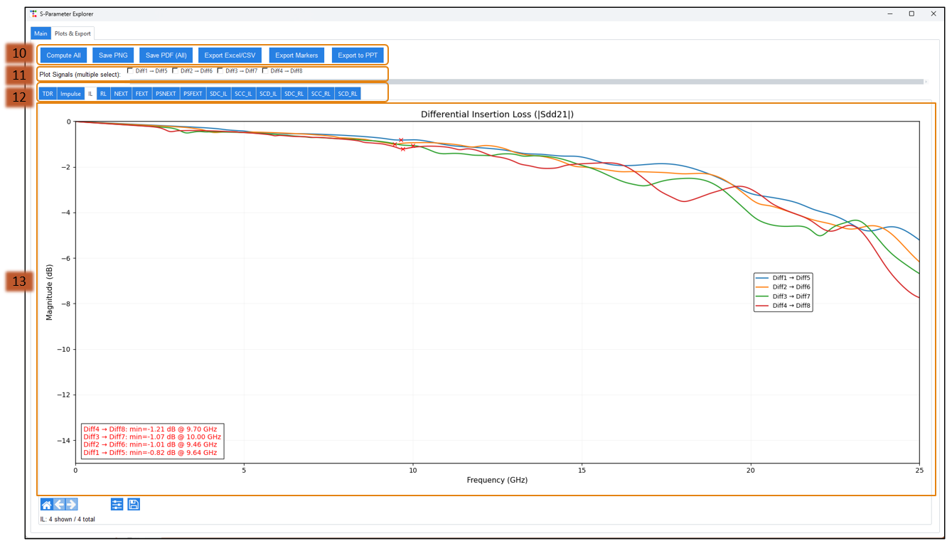
10. This window allows you to compute results, export plots, and generate reports.

10.1 Compute All:
Recomputes all results based on the options and configurations selected on the main page.

10.2 Save PNG:
Saves the currently displayed plot as a PNG file for documentation or later use.

10.3 Save PDF:
Exports all plots shown in the Results tab into a single PDF file.

10.4 Export Excel/CSV:
Exports all plotted data to Excel or CSV format for further analysis or offline processing.

10.5 Export Marker Data:
Exports the numerical data corresponding to all marker positions across all plots.

10.6 Export PPT:
Generates a PowerPoint file containing all plots along with a summary table showing worst-case values at the selected marker frequency, providing a compact and ready-to-share report.

11. Plot Signal (Multiple Select)

By default, all plots are displayed. Use this option to individually select only the plots you want to view.

12. Plots Window — Displays all analysis plots

TDR: Shows Time-Domain Reflectometry plots for single-ended and differential signals, including automatically determined minimum and maximum impedance.

Impulse Response: Displays the impulse response of the selected ports, including group delay and P/N skew.

IL (Insertion Loss):Shows insertion loss for differential or single-ended signals based on port mapping. Reports the worst 10 IL values at the marker frequency.

RL (Return Loss): Displays return loss for differential or single-ended signals. Reports the worst 10 RL values at the marker frequency.

NEXT (Near-End Crosstalk): Shows near-end crosstalk results and reports the worst 10 NEXT values at the marker frequency.

FEXT (Far-End Crosstalk): Displays far-end crosstalk and reports the worst 10 FEXT values at the marker frequency.

PSNEXT (Power-Sum NEXT):Shows power-sum near-end crosstalk and reports the worst 10 PSNEXT values at the marker frequency.

PSFEXT (Power-Sum FEXT):Displays power-sum far-end crosstalk and reports the worst 10 PSFEXT values at the marker frequency.

SDC / SCC / SCC IL: Displays:

SDC IL – Differential-to-common-mode IL

SCC IL – Common-to-differential-mode IL

CCC IL – Common-mode-to-common-mode IL Reports the worst 10 IL values at the marker frequency.

SDC / SCC / CCC RL: Displays:

SDC RL – Differential-to-common-mode RL

SCC RL – Common-to-differential-mode RL

CCC RL – Common-mode-to-common-mode RL Reports the worst 10 RL values at the marker frequency.

FAQs

What is s-parameter?

It’s a tool for analyzing electrical networks using scattering parameters.

How does viewer help?

The viewer plots multiple s-parameters like IL, RL, NEXT, and impulse response clearly.

What is s-parameter cascader?

It quickly combines multiple s-parameter files and shows advanced circuit visualization for easier understanding.

Our tools reduce workload and improve analysis speed.

Are more tools coming?

Is it user-friendly?

Yes, designed to be intuitive and easy for engineers.